Compare how different machine-learned interatomic potentials calculate silicon phonons with QuAcc and Rootstock

This example runs a materials science workflow with two different machine-learned interatomic potentials (MLIPs). We calculate phonon properties of crystalline silicon with the two MLIPs and see how they compare to each other and to experimental results.

We will use two SINAPSE SDK components:

• QuAcc provides the components of the computational materials science workflow.

• Rootstock provides the MLIPs that QuAcc will use at calculation time.

Prerequisites

You need an account on a cluster with a Rootstock installation. Check the Matter Model Almanac to see which are currently supported. The example will also assume that your allocation includes access to GPU time.

In a virtual environment, install the following packages:

$ pip install "quacc[phonons]" rootstock matplotlib

Note that you do not need to install PyTorch or individual MLIP packages because Rootstock manages pre-installed model environments on the cluster.

The phonon calculation workflow

This workflow takes a few minutes to run on a GPU node. Change CLUSTER to be the cluster you are running on, and double-check the Almanac to confirm the MLIPs you are using are available on your cluster.

"""Comparing how two MLIPs compute phonons of silicon using QuAcc + Rootstock."""

import json

from ase.build import bulk

from quacc.recipes.mlip.core import relax_job
from quacc.recipes.mlip.phonons import phonon_flow

# -- 1. Specify the cluster you're running on and the models to compare --
CLUSTER = "perlmutter"
CHECKPOINTS = {
    "mace-mh-1": {"head": "omat_pbe"},
    "orb-v3-conservative-inf-omat": {"precision": "float64"},
}

# -- 2. Build the structure ----------------------------------------------
atoms = bulk("Si")  # crystalline silicon

summary = {}
for checkpoint, setup_kwargs in CHECKPOINTS.items():
    # The "library" parameter tells QuAcc to use Rootstock.
    # The other parameters are passed to the Rootstock ASE calculator
    #   to load the right MLIP.
    common = {
        "library": "rootstock",
        "cluster": CLUSTER,
        "checkpoint": checkpoint,
        "device": "cuda",
        "setup_kwargs": setup_kwargs,
    }

    # -- 3. Make sure the structure is tightly relaxed before running phonons ----
    relaxed = relax_job(
        atoms, relax_cell=True, opt_params={"fmax": 1e-3}, **common
    )

    # -- 4. Use QuAcc's phonon flow, which calls phonopy -------
    phonons = phonon_flow(
        relaxed["atoms"],
        job_params={"static_job": common},
    )

    # -- 5. Prepare data for visualization -----------
    dos = phonons["results"]["total_dos"]
    thermal = phonons["results"]["thermal_properties"]
    summary[checkpoint] = {
        "dos_frequency_THz": dos["frequency_points"].tolist(),
        "dos": dos["total_dos"].tolist(),
        "temperature_K": thermal["temperatures"].tolist(),
        "heat_capacity_J_per_molK": thermal["heat_capacity"].tolist(),
        "free_energy_kJ_per_mol": thermal["free_energy"].tolist(),
    }
    print(f"{checkpoint}: done")

with open("phonon_summary.json", "w") as f:
    json.dump(summary, f)
print("Wrote phonon_summary.json")

Plot the comparison

With the output in phonon_summary.json, we can plot the phonon density of states and constant-volume heat capacity obtained with each MLIP. We also overlay experimental measurements from the literature for reference.

plot_phonons.py — click to expand

"""Plot the phonon comparison in phonon_summary.json against experiment."""

import json

import matplotlib.pyplot as plt

with open("phonon_summary.json") as f:
    summary = json.load(f)

# Experimental reference points. Frequency: the transverse-acoustic
# zone-boundary phonon from inelastic neutron scattering (Nilsson & Nelin,
# Phys. Rev. B 6, 3777 (1972), https://doi.org/10.1103/PhysRevB.6.3777).
# Heat capacity: NIST-JANAF values for crystalline Si
# (https://janaf.nist.gov/tables/Si-002.html), tabulated per mole of
# atoms (C_p, near-identical to C_V except at high temperature, where
# thermal expansion pushes it up).
EXP_FREQS_THZ = {"TA(X)": 4.49}
JANAF_T_K = [100, 200, 298.15, 400, 500, 600, 800, 1000]
JANAF_CP_PER_MOL_ATOMS = [7.268, 15.636, 20.000, 22.142, 23.330, 24.154,
                          25.359, 26.338]

COLORS = ["#2a78d6", "#eb6834", "#1baf7a"]  # colorblind-safe triple
INK, MUTED, GRID = "#0b0b0b", "#52514e", "#e1e0d9"

fig, (ax_dos, ax_cv) = plt.subplots(1, 2, figsize=(9.5, 3.8), dpi=200)

for color, (name, data) in zip(COLORS, summary.items()):
    ax_dos.plot(data["dos_frequency_THz"], data["dos"],
                color=color, lw=2, label=name)
    ax_cv.plot(data["temperature_K"], data["heat_capacity_J_per_molK"],
               color=color, lw=2, label=name)

# At high temperature every simple solid stores ~25 J/mol/K of heat per
# mole of atoms (the Dulong-Petit law): 3 vibration directions x the gas
# constant. phonopy reports per mole of cells, and our cell has 2 atoms.
GAS_CONSTANT = 8.314  # J/(mol K)
ATOMS_PER_CELL = 2    # bulk("Si") in the workflow script
dulong_petit = 3 * ATOMS_PER_CELL * GAS_CONSTANT
ax_cv.axhline(dulong_petit, color=MUTED, lw=1, ls=(0, (4, 4)))
ax_cv.text(0.98, dulong_petit, "Dulong–Petit  ", color=MUTED,
           fontsize=8, ha="right", va="bottom",
           transform=ax_cv.get_yaxis_transform())

# Experimental markers: dotted lines on the DOS, open circles on C_V.
for label, freq in EXP_FREQS_THZ.items():
    ax_dos.axvline(freq, color=MUTED, lw=1, ls=(0, (2, 3)))
    ax_dos.text(freq, 0.97, f"{label} ", color=MUTED, fontsize=8,
                ha="right", va="top", rotation=90,
                transform=ax_dos.get_xaxis_transform())
ax_cv.scatter(JANAF_T_K,
              [ATOMS_PER_CELL * cp for cp in JANAF_CP_PER_MOL_ATOMS],
              s=18, facecolors="none", edgecolors=INK, lw=1,
              zorder=3, label="experimental values")

ax_dos.set_xlabel("Frequency (THz)", color=MUTED)
ax_dos.set_ylabel("Phonon DOS (states/THz)", color=MUTED)
ax_dos.set_title("Si phonon density of states", color=INK, fontsize=10)
ax_cv.set_xlabel("Temperature (K)", color=MUTED)
ax_cv.set_ylabel("$C_V$ (J mol$^{-1}$ K$^{-1}$)", color=MUTED)
ax_cv.set_title("Heat capacity", color=INK, fontsize=10)
# One legend for both panels, in the heat-capacity panel's empty corner.
ax_cv.legend(frameon=False, fontsize=8, loc="lower right")

for ax in (ax_dos, ax_cv):
    ax.grid(color=GRID, lw=0.8)
    ax.set_axisbelow(True)
    for side in ("top", "right"):
        ax.spines[side].set_visible(False)
    ax.tick_params(colors=MUTED, labelsize=8)

fig.tight_layout()
fig.savefig("phonon_comparison.png", bbox_inches="tight")
print("Wrote phonon_comparison.png")

Results

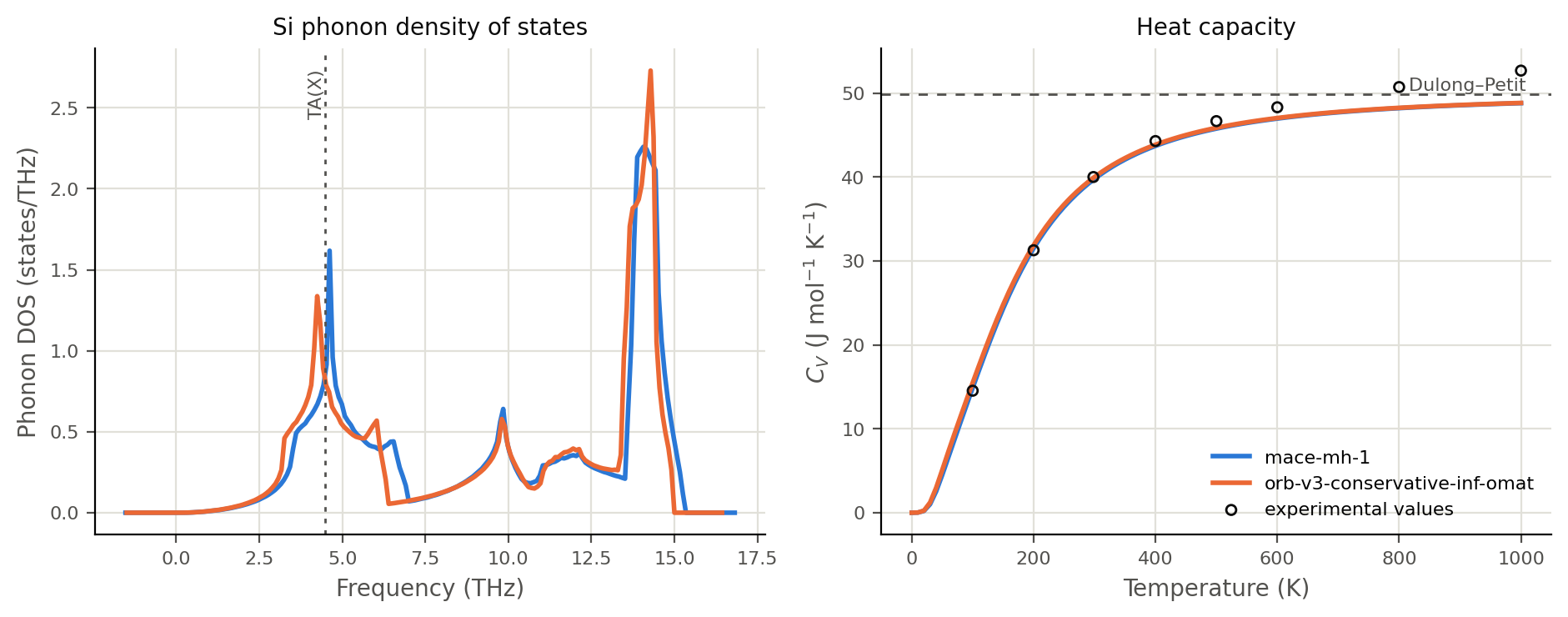
Experimental data: TA(X) phonon frequency from inelastic neutron scattering (Nilsson & Nelin, Phys. Rev. B 6, 3777 (1972)); heat capacities of crystalline Si from the NIST-JANAF Thermochemical Tables (Chase, 1998).

Both models reproduce the shape of the measured silicon spectrum, and the heat-capacity curves roughly track the NIST-JANAF measurements.

The models line up very closely on heat capacity, but have some noteworthy disagreement in the density of states. In particular, MACE-MH-1 (with the omat_pbe task head activated) places the transverse-acoustic peak at ~4.6 THz and Orb places it at ~4.2 THz, overshooting and undershooting the neutron-measured 4.5 THz respectively. This demonstrates that even when different MLIPs closely agree on some properties, they can disagree on zero-point vibrational energies in a way that would affect follow-on calculations of free energies.